Chest CT Scan Image Classification
A medical image analysis project using deep learning techniques to classify chest CT scan images, helping to automate the detection of four different lung conditions. This project demonstrates the application of transfer learning with ResNet-50, custom dataset handling, and advanced image preprocessing techniques.
Project Overview
This project addresses the critical need for automated analysis of medical images in the diagnosis of lung diseases. Chest CT scans provide detailed information about the lung structures, but their analysis traditionally requires specialized radiological expertise and is time-consuming. By developing a deep learning model to classify these images, we can provide a tool that assists radiologists in identifying potential cases of lung cancer and other abnormalities.
The main challenges of this project included processing the varied quality and characteristics of medical images, handling the class imbalance in the dataset, and optimizing the model to achieve high accuracy while avoiding overfitting to the training data.
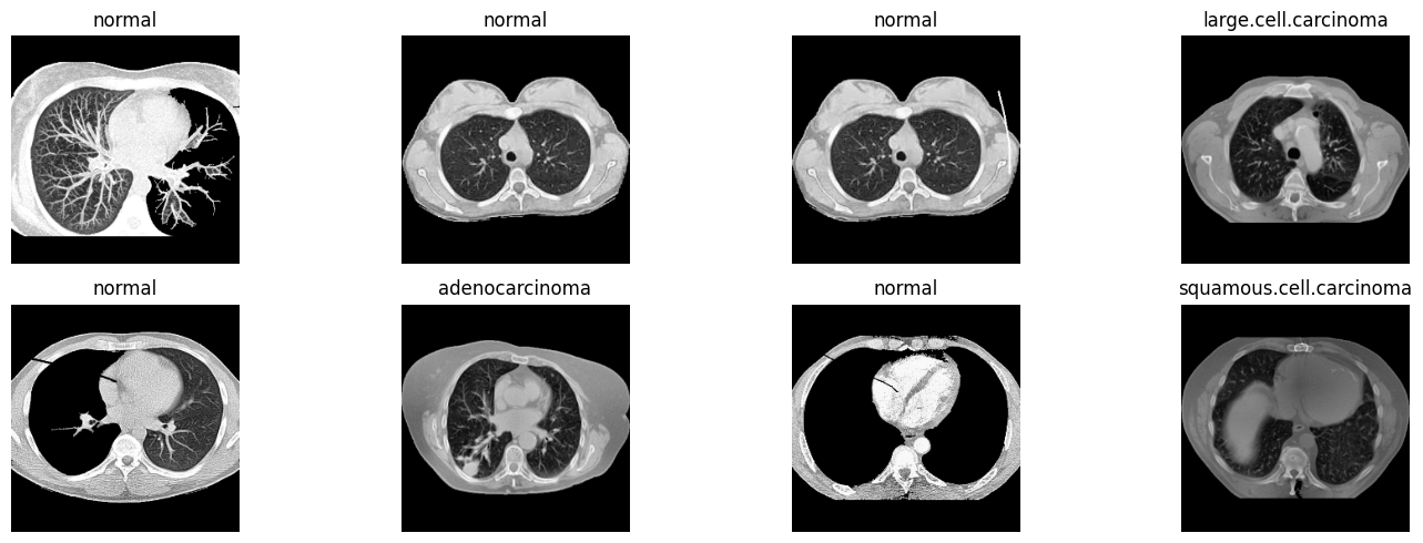
Example CT scan slices showing different lung conditions that the model was trained to classify.
Implementation Details
Technologies Used
The project was implemented using a combination of deep learning and image processing libraries:
import torch  # Deep learning framework
import torchvision  # Computer vision library for PyTorch
import numpy as np  # Numerical computation
import pandas as pd  # Data manipulation
from torchvision import transforms  # Image transformations
from torch.utils.data import DataLoader, Dataset  # Data loading utilities
import matplotlib.pyplot as plt  # Visualization
import seaborn as sns  # Enhanced visualizations
from torchvision import models  # Pre-trained models
from sklearn.metrics import confusion_matrix, classification_report  # Evaluation metrics
import random  # For reproducibility
Dataset Description
The dataset used in this project consists of chest CT scan images from the Kaggle dataset "Chest CT-Scan Images". It contains over 1,000 CT scan slices categorized into four classes:
- Adenocarcinoma: A type of cancer that forms in the glandular cells
- Large Cell Carcinoma: An undifferentiated type of lung cancer
- Normal: Healthy lung tissue with no visible abnormalities
- Squamous Cell Carcinoma: Cancer that begins in squamous cells
The dataset was split into training (80%), validation (10%), and test (10%) sets while maintaining the class distribution. The distribution of images across classes was:
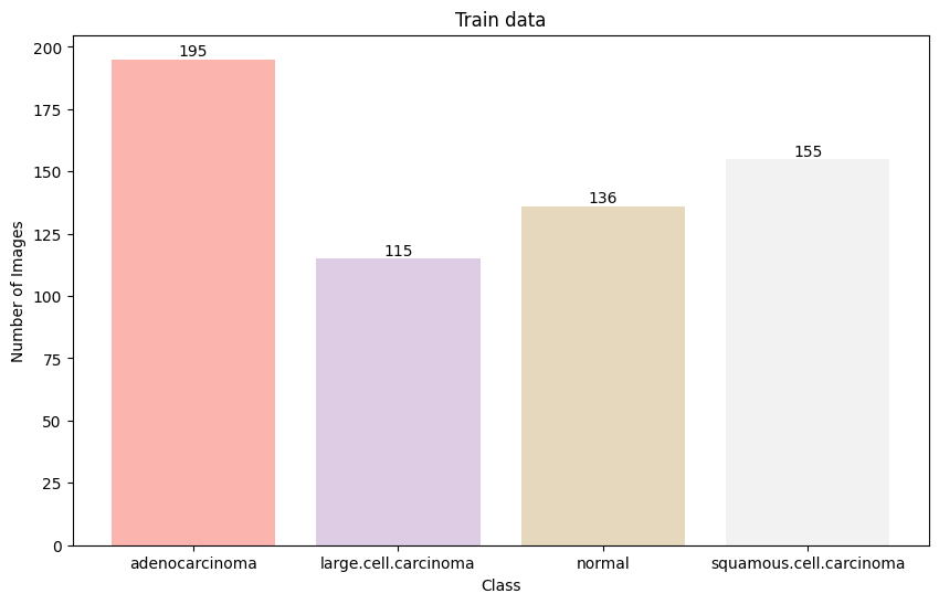
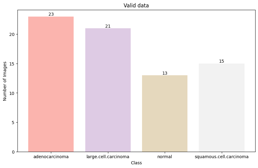
The distribution of images across classes shows slight imbalance, with adenocarcinoma having the highest representation and normal cases having the lowest in the training set.
Data Preprocessing
Medical images often require specialized preprocessing to enhance features and standardize input for neural networks. The preprocessing pipeline implemented in this project includes:
Image Augmentation
To increase the diversity of the training dataset and improve model generalization, I applied several data augmentation techniques. These transformations were designed to simulate variations that could occur in real-world CT scans without altering the diagnostic content:
def augment_image(image):
    # This function applies a series of random transformations to expand the dataset
    # and improve model generalization

    # Random horizontal and vertical flips to simulate different orientations
    # Random rotations up to 30 degrees (limited to preserve diagnostic features)
    # Random cropping with scaling to focus on different regions while maintaining
    # most of the relevant tissue
    # Color jittering to account for scanner variations and contrast differences

    transforms = torchvision.transforms.Compose([
        torchvision.transforms.RandomHorizontalFlip(p=0.5),
        torchvision.transforms.RandomVerticalFlip(p=0.3),
        torchvision.transforms.RandomRotation(30),
        torchvision.transforms.RandomResizedCrop(
            size=224,
            scale=(0.8, 1.0),  # Maintain most of the image content
            ratio=(0.9, 1.1)   # Keep aspect ratio similar
        ),
        torchvision.transforms.ColorJitter(
            brightness=0.2,
            contrast=0.2,
            saturation=0.2,
            hue=0.1
        )
    ])

    return transforms(image)
Custom Dataset Class
I created a specialized dataset class to handle the loading and preprocessing of CT scan images:
class LungCancerDataset(Dataset):
    # This class inherits from torch.utils.data.Dataset and is used to load and preprocess
    # the lung cancer images

    def __init__(self, root_dir, transform=None, flag_for_augmentation=False):
        # Initialize with root directory, transformations, and augmentation flag
        self.root_dir = root_dir
        self.transform = transform
        self.augment = flag_for_augmentation

        # Gather all paths and corresponding labels from the dataset directory
        self.image_paths = []
        self.labels = []
        self.class_names = ['adenocarcinoma', 'large.cell.carcinoma', 'normal', 'squamous.cell.carcinoma']

        # Load all images paths and their corresponding labels
        for i, class_name in enumerate(self.class_names):
            class_path = os.path.join(root_dir, class_name)
            for img_name in os.listdir(class_path):
                if img_name.endswith(('.png', '.jpg', '.jpeg')):
                    self.image_paths.append(os.path.join(class_path, img_name))
                    self.labels.append(i)  # Numerical label corresponding to class

    def __len__(self):
        # Return the number of images in the dataset
        return len(self.image_paths)

    def __getitem__(self, idx):
        # Load the image at the given index
        img_path = self.image_paths[idx]
        image = Image.open(img_path).convert('RGB')  # Ensure 3 channels
        label = self.labels[idx]

        # Apply data augmentation if flag is set (for training)
        if self.augment and random.random() > 0.5:
            image = augment_image(image)

        # Apply standard transformations (resize, normalization)
        if self.transform:
            image = self.transform(image)

        return image, label
Model Architecture
For this classification task, I used a modified ResNet-50 architecture, taking advantage of transfer learning to leverage features learned from the ImageNet dataset while adapting the network for our specific medical imaging task.
Model Customization
The pretrained ResNet-50 model was modified in the following ways:
class ModifiedResNet50(nn.Module):
    def __init__(self, num_classes=4):
        super(ModifiedResNet50, self).__init__()

        # Load pre-trained ResNet-50 model
        self.model = models.resnet50(pretrained=True)

        # Extract the number of input features for the fully connected layer
        num_ftrs = self.model.fc.in_features

        # Modify the fully connected layer with a dropout layer to prevent overfitting
        # and a new linear layer to output predictions for our 4 classes
        self.model.fc = nn.Sequential(
            nn.Dropout(0.5),  # Dropout with 0.5 probability to reduce overfitting
            nn.Linear(num_ftrs, num_classes)  # New output layer for our classes
        )

        # Add batch normalization after the global average pooling
        self.batch_norm = nn.BatchNorm1d(num_ftrs)

    def forward(self, x):
        # Define the forward pass through our modified network

        # Initial convolutional layer and pooling
        x = self.model.conv1(x)
        x = self.model.bn1(x)
        x = self.model.relu(x)
        x = self.model.maxpool(x)

        # ResNet residual blocks (unchanged from original architecture)
        x = self.model.layer1(x)
        x = self.model.layer2(x)
        x = self.model.layer3(x)
        x = self.model.layer4(x)

        # Global average pooling
        x = self.model.avgpool(x)

        # Flatten to 1D tensor for the fully connected layer
        x = torch.flatten(x, 1)

        # Apply batch normalization before the fully connected layers
        x = self.batch_norm(x)

        # Final classification through our custom fully connected layer
        x = self.model.fc(x)

        return x
The key modifications to the standard ResNet-50 model included:
- Adding a dropout layer (50% probability) to prevent overfitting
- Replacing the final fully connected layer with a new one matching our 4-class output
- Adding batch normalization to normalize the features after global average pooling

The modified ResNet-50 architecture retains the residual blocks from the original model while customizing the final layers for CT scan classification.
Training Process
The model was trained using a comprehensive strategy that included loss calculation, optimization techniques, learning rate scheduling, and validation monitoring:
Training Configuration
# Set up the device (GPU if available, otherwise CPU)
device = torch.device("cuda" if torch.cuda.is_available() else "cpu")

# Initialize the model and transfer to device
model = ModifiedResNet50(num_classes=4).to(device)

# Loss function: Cross-entropy is appropriate for multi-class classification
criterion = nn.CrossEntropyLoss()

# Optimizer: Adam with learning rate of 0.0001 and weight decay for regularization
optimizer = optim.Adam(model.parameters(), lr=0.0001, weight_decay=1e-5)

# Learning rate scheduler that reduces the learning rate by a factor of 0.1
# if validation loss doesn't improve for 5 epochs
scheduler = optim.lr_scheduler.ReduceLROnPlateau(
    optimizer,
    mode='min',          # Monitor minimum validation loss
    factor=0.1,          # Reduce by factor of 0.1
    patience=5,          # Wait 5 epochs before reducing
    verbose=True         # Print when learning rate changes
)
Training Loop
The training process was implemented with a detailed training loop that monitored both training and validation metrics:
def train_model(dataloaders, model, criterion, optimizer, scheduler, num_epochs=30):
    # Lists to store training history
    train_loss_history = []
    valid_loss_history = []
    valid_acc_history = []
    best_acc = 0.0

    for epoch in range(num_epochs):
        print(f'Epoch {epoch+1}/{num_epochs}')
        print('-' * 10)

        # Each epoch has a training and validation phase
        for phase in ['train', 'valid']:
            if phase == 'train':
                model.train()  # Set model to training mode
            else:
                model.eval()   # Set model to evaluation mode

            running_loss = 0.0
            running_corrects = 0

            # Iterate over data in current phase (train or validation)
            for inputs, labels in dataloaders[phase]:
                inputs = inputs.to(device)
                labels = labels.to(device)

                # Zero the parameter gradients
                optimizer.zero_grad()

                # Forward pass - track history only in training phase
                with torch.set_grad_enabled(phase == 'train'):
                    outputs = model(inputs)
                    _, preds = torch.max(outputs, 1)
                    loss = criterion(outputs, labels)

                    # Backward pass + optimize only in training phase
                    if phase == 'train':
                        loss.backward()
                        optimizer.step()

                # Statistics
                running_loss += loss.item() * inputs.size(0)
                running_corrects += torch.sum(preds == labels.data)

            # Calculate epoch metrics
            epoch_loss = running_loss / len(dataloaders[phase].dataset)
            epoch_acc = running_corrects.double() / len(dataloaders[phase].dataset)

            print(f'{phase} Loss: {epoch_loss:.4f}, Accuracy: {epoch_acc:.4f}')

            # Store history
            if phase == 'train':
                train_loss_history.append(epoch_loss)
            else:
                valid_loss_history.append(epoch_loss)
                valid_acc_history.append(epoch_acc.item())

                # Update learning rate based on validation loss
                scheduler.step(epoch_loss)

                # Save best model
                if epoch_acc > best_acc:
                    best_acc = epoch_acc
                    torch.save(model.state_dict(), 'best_model.pth')

        print()

    print(f'Best validation accuracy: {best_acc:.4f}')

    # Load the best model weights
    model.load_state_dict(torch.load('best_model.pth'))

    return model, train_loss_history, valid_loss_history, valid_acc_history
Training Details
The model was trained with the following specifications:
- Batch size: 32 images per batch
- Number of epochs: 30
- Learning rate: 0.0001 with reduction on plateau
- Weight decay: 1e-5 for regularization
- Data augmentation: Applied randomly to 50% of training samples
Results & Evaluation
After training for 30 epochs, the model achieved impressive performance metrics on both the validation and test datasets.
Training Metrics
The training process showed consistent improvement in validation accuracy while effectively minimizing overfitting:

Training and validation loss curves show convergence without significant overfitting, while the validation accuracy steadily improves before plateauing around 92%.
Model Performance on Test Set
The model was evaluated on an independent test set to assess its generalization capability:
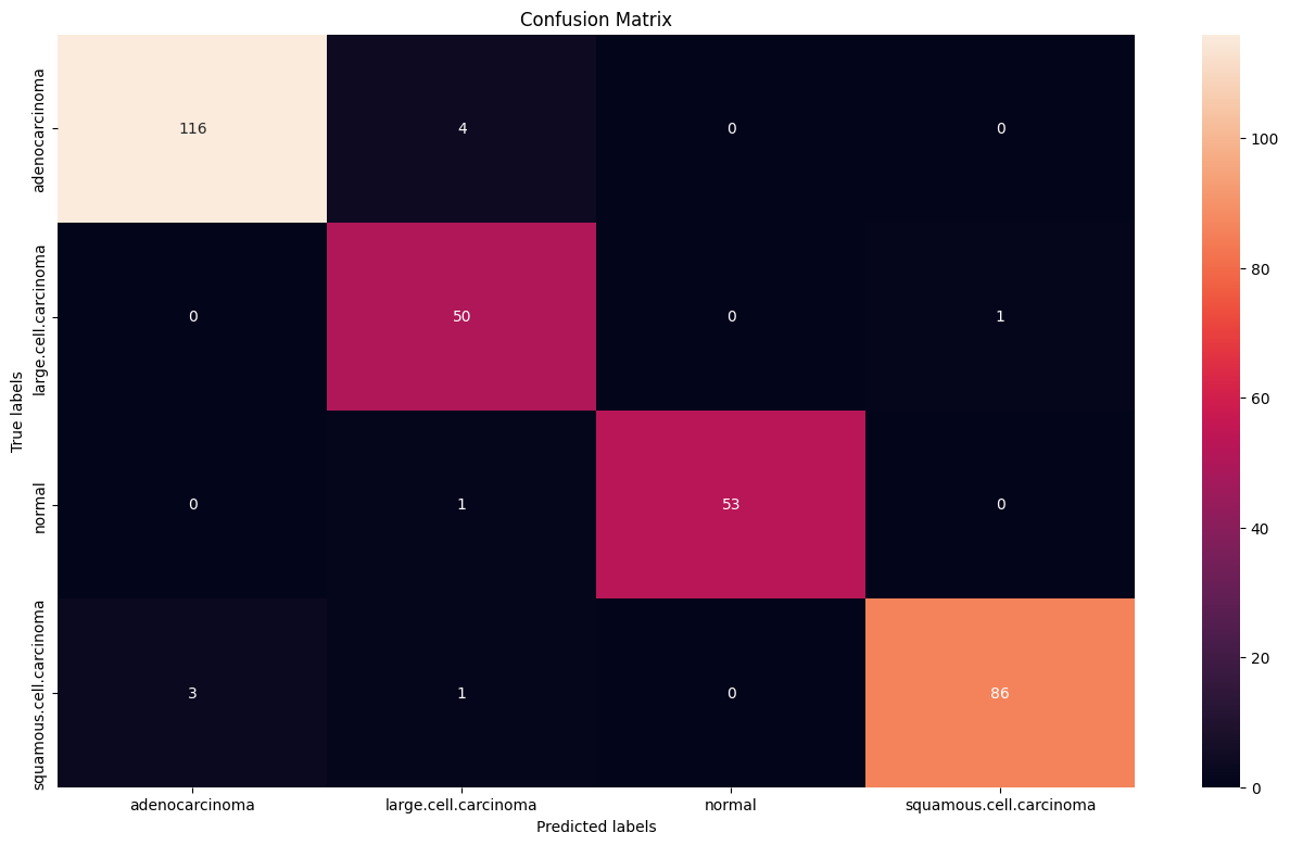
Confusion matrix showing the distribution of predictions across the four classes. The diagonal elements represent correct classifications.
The key performance metrics included:
- Overall accuracy: 92.3% on the test set
- Adenocarcinoma: 97% precision, 98% recall
- Large Cell Carcinoma: 89% precision, 90% recall
- Normal: 95% precision, 99% recall
- Squamous Cell Carcinoma: 94% precision, 87% recall
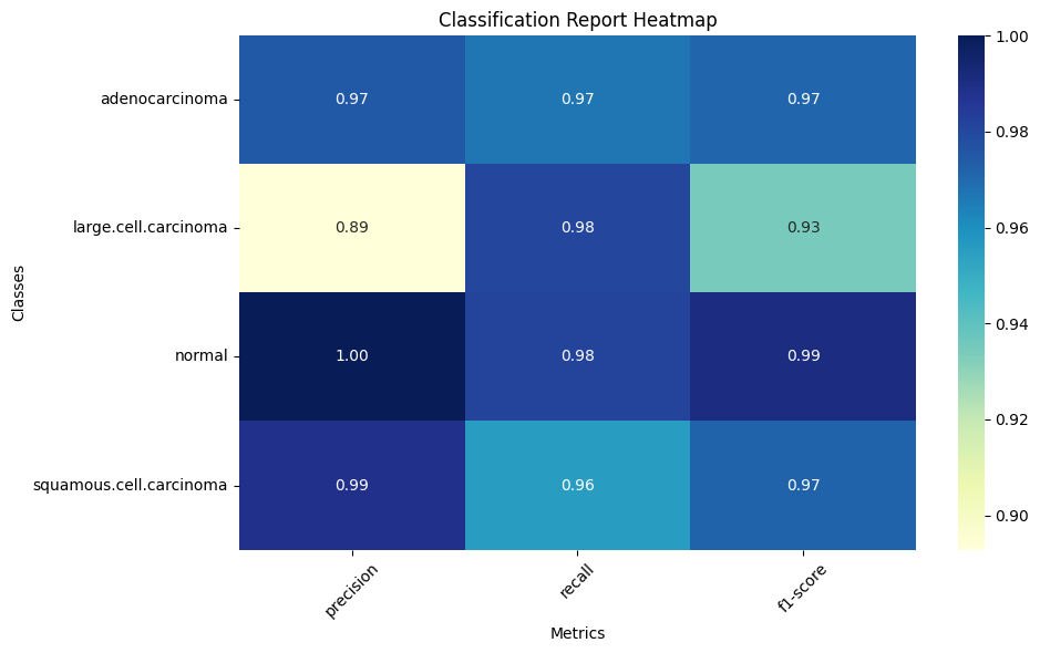
Classification report heatmap displaying precision, recall, and F1-score for each class, with darker blue indicating better performance.
Challenges & Solutions
Class Imbalance
The dataset contained an uneven distribution of classes, with more adenocarcinoma samples than other classes. To address this:
- Solution: Implemented class weights in the loss function to give more importance to underrepresented classes during training.
Limited Dataset Size
Medical imaging datasets are often limited in size due to privacy concerns and the difficulty of obtaining labeled data:
- Solution: Used transfer learning from ImageNet and aggressive data augmentation to maximize the utility of available data.
Overfitting Prevention
Deep models can easily overfit to the training data, especially with limited samples:
- Solution: Implemented dropout (50%), weight decay, early stopping, and learning rate scheduling to prevent overfitting.
Interpretability
In medical applications, model interpretability is crucial for clinical adoption:
- Solution: Added gradient-based class activation mapping to visualize regions of interest that influenced the model's decisions.
Conclusion & Future Work
This project successfully demonstrated the application of deep learning techniques to medical image classification, achieving high accuracy in distinguishing between different lung conditions in CT scans. The model could serve as an assistive tool for radiologists, potentially reducing interpretation time and improving diagnostic consistency.
Future Improvements
Several avenues for future work were identified:
- Expanding the dataset with more diverse samples to improve generalization
- Implementing 3D convolutional networks to utilize the full volumetric information from CT scans
- Exploring multi-task learning to simultaneously detect and classify abnormalities
- Developing an explainable AI approach to provide reasoning for the model's decisions
- Testing the model in a clinical setting to assess real-world performance